1 Activation Functions

1.1 Activation Functions

1.1.1 Overview & Motivation

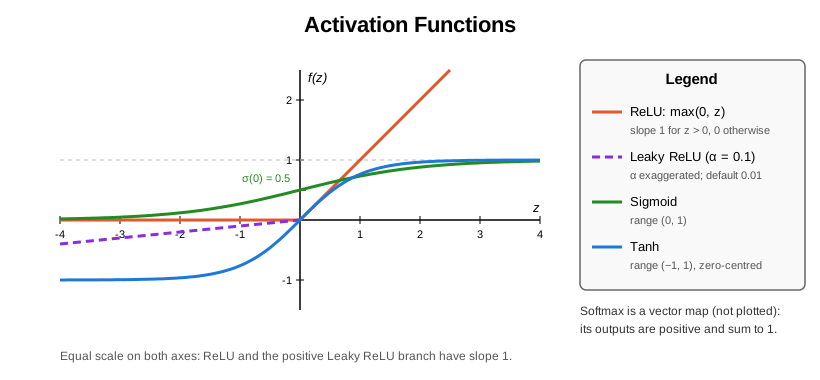
An activation function \(f\) is the non-linear transformation applied after the affine map in each neural network layer:

\[a = f(z) = f(W x + b)\]

Without activation functions, stacking layers would collapse into a single affine transformation — the network could only represent linear mappings regardless of depth. Activation functions are what give neural networks their expressive power.

The choice of activation function controls gradient flow during back-propagation, output range, and computational cost — all critical on resource-constrained embedded targets.

1.1.2 Mathematical Theory

1.1.2.1 Forward and Backward

Every activation function provides two operations on a pre-activation vector \(z \in \mathbb{R}^k\) with output \(a = f(z)\):

\(J_f(z) = \partial a / \partial z\) is the \(k \times k\) Jacobian. For the element-wise functions (ReLU, Leaky ReLU, Sigmoid, Tanh), \(a_i\) depends only on \(z_i\), so the Jacobian is diagonal and the backward pass reduces to a Hadamard product:

\[\delta = g \odot f'(z), \qquad \delta_i = g_i \, f'(z_i)\]

For Softmax, every output depends on every input, so the Jacobian is dense; the backward pass is still computed in \(O(k)\) as a Jacobian-vector product (see Softmax). The derivatives of Sigmoid and Tanh are written in terms of the output \(a\), so the backward pass reuses the cached forward result instead of re-evaluating the exponential.

1.1.2.2 Catalogue

1.1.2.2.1 ReLU

\[f(z) = \max(0, z), \qquad f'(z) = \begin{cases} 1 & z > 0 \\ 0 & z \le 0 \end{cases}\]

• Computationally cheapest (single comparison).
• Sparse activations accelerate training.
• Risk: neurons with \(z \le 0\) for all inputs are permanently dead.

1.1.2.2.2 Leaky ReLU

\[f(z) = \begin{cases} z & z > 0 \\ \alpha z & z \le 0 \end{cases}, \qquad f'(z) = \begin{cases} 1 & z > 0 \\ \alpha & z \le 0 \end{cases}\]

where \(\alpha \in [0, 1)\) is a small constant (default \(0.01\)). Prevents dead neurons by allowing a small gradient for \(z < 0\); \(\alpha = 0\) reduces to ReLU.

1.1.2.2.3 Sigmoid

\[f(z) = \frac{1}{1 + e^{-z}}, \qquad f'(z) = f(z)\,\bigl(1 - f(z)\bigr)\]

• Output range \((0, 1)\) with \(f(0) = 0.5\) — natural for probabilities.
• Maximum slope \(f'(0) = 0.25\).
• Risk: saturates for \(|z| \gg 0\), causing vanishing gradients.

The naive formula overflows \(e^{-z}\) for large negative \(z\). The numerically stable evaluation branches on the sign so the exponent is never positive:

\[f(z) = \begin{cases} \dfrac{1}{1 + e^{-z}} & z \ge 0 \\[2ex] \dfrac{e^{z}}{1 + e^{z}} & z < 0 \end{cases}\]

Both branches are the same function; each only evaluates \(e^{-|z|} \in (0, 1]\).

1.1.2.2.4 Tanh

\[f(z) = \tanh(z) = \frac{e^z - e^{-z}}{e^z + e^{-z}}, \qquad f'(z) = 1 - f(z)^2\]

• Output range \((-1, 1)\) — zero-centered, unlike Sigmoid; \(f'(0) = 1\).
• Same saturation problem as Sigmoid at extremes.
• \(\tanh(z) = 2\sigma(2z) - 1\), so it inherits Sigmoid’s saturation behaviour.

1.1.2.2.5 Softmax

For a vector \(z \in \mathbb{R}^k\):

\[a_i = f(z)_i = \frac{e^{z_i}}{\sum_{j=1}^{k} e^{z_j}}\]

• Outputs are strictly positive and form a probability distribution: \(\sum_i a_i = 1\).
• Shift invariant: \(f(z + c\mathbf{1}) = f(z)\) for any scalar \(c\). Evaluation subtracts \(z_{\max} = \max_j z_j\) first, so every exponent is \(\le 0\) and nothing overflows; the outputs are exact probabilities, with no clamping.
• Softmax is only meaningful on the whole vector. Applied to a single element (\(k = 1\)) it is the constant \(1\) with derivative \(0\).

Jacobian. Differentiating the quotient gives

\[\frac{\partial a_i}{\partial z_j} = a_i\,(\mathbb{1}[i = j] - a_j), \qquad J = \operatorname{diag}(a) - a\,a^T\]

Backward as a Jacobian-vector product. \(J\) is symmetric, so

\[\delta = J^T g = a \odot g - a\,(a^T g), \qquad \delta_i = a_i \Bigl(g_i - \sum_{k} g_k a_k\Bigr)\]

One dot product \(\langle g, a \rangle\) and one element-wise pass: \(O(k)\) time and \(O(1)\) extra space. The \(k \times k\) Jacobian is never formed.

1.1.3 Complexity Analysis

All activations need \(O(1)\) extra space beyond the input, output and gradient vectors the layer already holds.

1.1.4 Step-by-Step Walkthrough

Element-wise case. ReLU on the pre-activations \(z = [-0.5, \; 1.2, \; 0.0]\).

Forward:

Backward with incoming gradient \(g = \partial \mathcal{L} / \partial a = [0.3, \; -0.7, \; 0.1]\):

Neuron 1 is dead — its gradient is zero and its weights will not update. If this persists across all training samples, the neuron is permanently inactive.

Vector case. Softmax on \(z = [1.0, \; 2.0, \; 0.5]\) with upstream gradient \(g = [0.3, \; -0.2, \; 0.1]\).

The outputs sum to \(1\) and the gradient sums to \(0\) (\(\sum_i \delta_i = \langle g, a \rangle - \langle g, a \rangle \sum_i a_i = 0\)), reflecting the shift invariance.

1.1.5 Pitfalls & Edge Cases

• Vanishing gradients with Sigmoid/Tanh. For deep networks, gradients shrink exponentially through saturated activations. Use ReLU or Leaky ReLU in hidden layers.
• Dead ReLU neurons. If a neuron’s bias drifts negative enough that no input ever produces \(z > 0\), it stops learning. Leaky ReLU or He initialization prevents this.
• Exponential overflow. In single precision \(e^{z}\) overflows for \(z > 88.7\). Sigmoid is evaluated with the sign-branched form and Softmax with the max shift, so neither overflows for any finite input; the saturated outputs round to exactly \(0\) or \(1\), which makes the derivative \(0\) there.
• Softmax sums. After the max shift the largest exponential is exactly \(1\), so the normaliser is in \([1, k]\) and never underflows to zero. The outputs are not clamped: clamping each probability would break \(\sum_i a_i = 1\) and make the backward pass inconsistent with the forward pass.
• Softmax is not element-wise. Its scalar form is degenerate (constant \(1\), derivative \(0\)); only the vector form is meaningful. Do not place a Softmax output in front of a loss that already applies softmax to its input (see Loss Functions).
• Non-differentiable points. ReLU and Leaky ReLU are not differentiable at \(z = 0\); the sub-gradient \(f'(0) = 0\) (ReLU) and \(f'(0) = \alpha\) (Leaky ReLU) is used.
• Fast-math builds. Aggressive floating-point optimisation may assume finite values; non-finite inputs (NaN, \(\pm\infty\)) are outside the contract of every activation.

1.1.6 Variants & Generalizations

1.1.7 Applications

• Hidden layers — ReLU (or Leaky ReLU) is the default choice for feed-forward and convolutional hidden layers.
• Binary classification output — Sigmoid maps the output to a probability for binary cross-entropy.
• Multi-class probabilities — Softmax produces a probability distribution when probabilities are the desired output (inference, reporting).
• Recurrent networks — Tanh is traditionally used in LSTM/GRU gates.
• Embedded inference — Hard Sigmoid/Tanh avoid expensive exponentials on MCUs without FPU.

1.1.8 Connections to Other Algorithms

graph TD
    Act["Activation Functions"]
    Layer["Dense Layer"]
    NN["Neural Network"]
    Loss["Loss Functions"]
    Act --> Layer
    Layer --> NN
    NN --> Loss

2 Layers

2.1 Dense Layer

2.1.1 Overview & Motivation

A dense (fully-connected) layer is the most fundamental building block of a neural network. It maps an input vector \(a_{\text{in}} \in \mathbb{R}^n\) to an output vector \(a_{\text{out}} \in \mathbb{R}^m\) through a learnable affine transformation followed by an activation function:

\[a_{\text{out}} = f(W \, a_{\text{in}} + b)\]

Every input neuron is connected to every output neuron — hence “fully connected.” The layer’s parameters are the weight matrix \(W\) and bias vector \(b\); training adjusts these to minimize the loss.

In this library, input size, output size, and parameter count are all compile-time constants, enabling static allocation and dimension checking with zero runtime overhead. The caller supplies the initial weights; the biases start at zero.

2.1.2 Mathematical Theory

2.1.2.1 Forward Pass

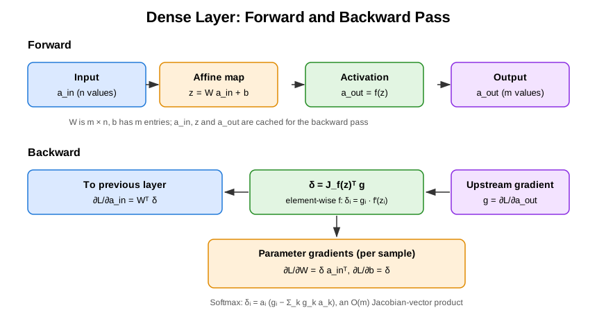
\[z = W \, a_{\text{in}} + b, \qquad a_{\text{out}} = f(z)\]

where \(W \in \mathbb{R}^{m \times n}\), \(b \in \mathbb{R}^m\), and \(f\) is the activation function. The layer caches \(a_{\text{in}}\), \(z\) and \(a_{\text{out}}\) for the backward pass.

2.1.2.2 Backward Pass

Given the upstream gradient \(g = \partial \mathcal{L} / \partial a_{\text{out}} \in \mathbb{R}^m\) for one sample:

1. Pre-activation gradient — the transposed activation Jacobian applied to \(g\): \[\delta = \frac{\partial \mathcal{L}}{\partial z} = J_f(z)^T g\] For an element-wise activation the Jacobian is diagonal and this reduces to \(\delta = g \odot f'(z)\). For Softmax it is \(\delta_i = a_i \bigl(g_i - \sum_k g_k a_k\bigr)\) with \(a = a_{\text{out}}\), still \(O(m)\) (see Softmax).

2. Weight gradient: \[\frac{\partial \mathcal{L}}{\partial W} = \delta \, a_{\text{in}}^T\]

3. Bias gradient: \[\frac{\partial \mathcal{L}}{\partial b} = \delta\]

4. Input gradient (propagated to the previous layer): \[\frac{\partial \mathcal{L}}{\partial a_{\text{in}}} = W^T \delta\]

The backward pass requires a preceding forward pass (it uses the cached \(a_{\text{in}}\), \(z\), \(a_{\text{out}}\)). Each call overwrites the stored parameter gradients with those of the current sample; they are not accumulated and are not yet exposed to an optimizer (roadmap N8).

2.1.2.3 Parameter Vector

The parameters are stored as one flat vector: \(W\) in row-major order (row \(i\) holds the weights of output neuron \(i\)) followed by \(b\):

\[\theta = [\, W_{1,1}, \ldots, W_{1,n}, \; W_{2,1}, \ldots, W_{m,n}, \; b_1, \ldots, b_m \,], \qquad P = m\,n + m = m(n + 1)\]

For a layer with 128 inputs and 64 outputs: \(P = 64 \times 129 = 8{,}256\) parameters.

2.1.3 Complexity Analysis

The matrix-vector products dominate both passes. For embedded networks (e.g. \(n = 32, m = 16\)), a single forward pass takes 512 multiply-accumulate operations.

Resident memory per layer. The object holds the parameters (\(P\) values), a parameter-gradient buffer of the same size (\(P\)), and the cached input, pre-activation, output and input-gradient vectors (\(2n + 2m\)):

\[\text{values} = 2P + 2n + 2m = 2mn + 4m + 2n\]

That is roughly twice the weight matrix. A \(256 \times 256\) float layer holds \(2 \times 65{,}792 + 1{,}024 = 132{,}608\) values, about \(518\,\text{KiB}\) — not the \(256\,\text{KiB}\) of the weights alone. The model adds a transient \(P\)-sized copy when parameters are exported or imported.

2.1.4 Step-by-Step Walkthrough

Layer: 3 inputs → 2 outputs, ReLU activation.

\[W = \begin{bmatrix} 0.5 & -0.3 & 0.8 \\ 0.1 & 0.7 & -0.2 \end{bmatrix}, \quad b = \begin{bmatrix} 0.1 \\ -0.1 \end{bmatrix}, \quad a_{\text{in}} = \begin{bmatrix} 1.0 \\ 0.5 \\ -1.0 \end{bmatrix}\]

Forward:

Backward with \(g = \partial \mathcal{L} / \partial a_{\text{out}} = [0.2,\; -0.4]^T\):

In the flat parameter layout, \(\nabla\theta = [0, 0, 0, -0.4, -0.2, 0.4, 0, -0.4]\).

2.1.5 Pitfalls & Edge Cases

• Dimension mismatch. In a multi-layer network, the output size of layer \(\ell\) must equal the input size of layer \(\ell+1\). This library enforces this at compile time.
• Weight initialization. The caller supplies the initial weights. Zero or identical weights make all neurons compute the same thing (symmetry problem). For ReLU layers use He initialization, \(W_{ij} \sim \mathcal{N}(0,\, 2/n_{\text{in}})\) — variance \(2/n_{\text{in}}\), standard deviation \(\sqrt{2/n_{\text{in}}}\), with \(n_{\text{in}} = n\) the fan-in. For Sigmoid/Tanh use Glorot, \(\operatorname{Var}(W_{ij}) = 2/(n_{\text{in}} + n_{\text{out}})\).
• Backward before forward. The backward pass uses the caches of the most recent forward pass; calling it first is a precondition violation.
• Per-sample gradients. Each backward pass overwrites the parameter gradients. Mini-batch training must sum them across samples itself; accumulation and gradient export are roadmap N8 and N16.
• Softmax in a hidden or output layer. Supported through its Jacobian-vector product, but do not feed a Softmax output into categorical cross-entropy, which expects logits (see Loss Functions).
• Large layers exhaust RAM. The resident footprint is about \(2P\) values plus caches (see Complexity Analysis). A \(256 \times 256\) float layer needs about 518 KiB; place large layers in statically allocated memory sized for that, not on a small task stack.
• Accumulation error. The dot product of \(n\) single-precision terms accumulates rounding error of order \(n \varepsilon\) in the worst case; keep inputs normalised to similar magnitudes.

2.1.6 Variants & Generalizations

2.1.7 Applications

• Hidden layers — One or more dense layers form the core of feed-forward networks for regression and classification.
• Output layer — A final dense layer maps to the target dimensionality (1 for regression, \(k\) for \(k\)-class classification).
• Embedding projection — Dense layers project high-dimensional sparse inputs to low-dimensional dense representations.
• Controller networks — In neural network-based control, small dense layers map state vectors to actuator commands.

2.1.8 Connections to Other Algorithms

graph TD
    Layer["Dense Layer"]
    Act["Activation Functions"]
    Model["Model"]
    Opt["Optimizer"]
    LR["Linear Regression"]

    Act --> Layer
    Layer --> Model
    Model --> Opt
    Layer -.->|"identity activation, MSE loss"| LR

3 Loss Functions

3.1 Loss Functions

3.1.1 Overview & Motivation

A loss function \(\mathcal{L}(\hat{y}, y)\) quantifies how far a model’s prediction \(\hat{y}\) is from the true target \(y\). Training a neural network means finding parameters \(\theta\) that minimize the expected loss over the training data:

\[\theta^* = \arg\min_\theta \; \mathbb{E}[\mathcal{L}(f_\theta(x), y)]\]

The loss function defines the entire learning objective — different losses lead to different optimal models even on the same data. It must also provide the gradient \(\nabla_{\hat{y}} \mathcal{L}\) that seeds back-propagation.

In this library every loss is an objective over one vector argument \(v \in \mathbb{R}^N\) — the \(N\) outputs of one sample — compared against a target \(y \in \mathbb{R}^N\) fixed when the loss is created. A regularization term \(R\) from numerical-toolbox-cpp is added to the same argument:

\[J(v) = \mathcal{L}(v, y) + R(v), \qquad \nabla J(v) = \nabla_v \mathcal{L}(v, y) + \nabla R(v)\]

For MSE, MAE and BCE the argument is the prediction \(v = \hat{y}\); for categorical cross-entropy it is the vector of logits \(v = z\).

3.1.2 Mathematical Theory

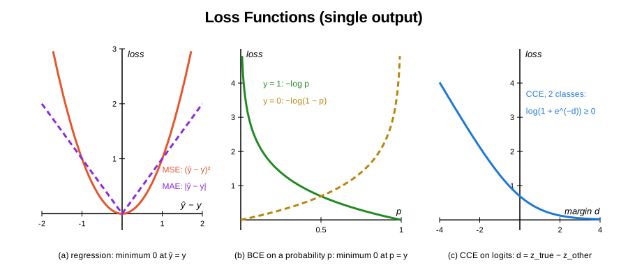
All data terms are means over the \(N\) outputs, so their gradients carry a \(1/N\) factor.

3.1.2.1 Mean Squared Error

\[\mathcal{L}_{\text{MSE}} = \frac{1}{N} \sum_{i=1}^{N} (\hat{y}_i - y_i)^2, \qquad \frac{\partial \mathcal{L}}{\partial \hat{y}_i} = \frac{2}{N}(\hat{y}_i - y_i)\]

• Penalizes large errors quadratically → sensitive to outliers.
• Natural choice for regression tasks; maximum-likelihood under Gaussian noise.

3.1.2.2 Mean Absolute Error

\[\mathcal{L}_{\text{MAE}} = \frac{1}{N} \sum_{i=1}^{N} |\hat{y}_i - y_i|, \qquad \frac{\partial \mathcal{L}}{\partial \hat{y}_i} = \frac{1}{N} \operatorname{sign}(\hat{y}_i - y_i)\]

• Linear penalty → robust to outliers; maximum-likelihood under Laplacian noise.
• Not differentiable at \(\hat{y}_i = y_i\); the sub-gradient \(\operatorname{sign}(0) = 0\) is used there, so an exact fit is a stationary point.

3.1.2.3 Binary Cross-Entropy

The input is a vector of probabilities \(p = \hat{y} \in [0, 1]^N\) (e.g. a Sigmoid output) and \(y_i \in [0, 1]\). Each probability is first clamped to \(\tilde{p}_i = \operatorname{clamp}(p_i, \varepsilon, 1 - \varepsilon)\) with \(\varepsilon = 10^{-7}\):

\[\mathcal{L}_{\text{BCE}} = -\frac{1}{N}\sum_{i=1}^{N} \left[ y_i \log \tilde{p}_i + (1 - y_i) \log(1 - \tilde{p}_i) \right]\]

\[\frac{\partial \mathcal{L}}{\partial p_i} = \frac{1}{N} \cdot \frac{\tilde{p}_i - y_i}{\tilde{p}_i(1 - \tilde{p}_i)}\]

• The clamp keeps both logarithms finite: each term is at most \(-\log \varepsilon \approx 16.1\).
• The gradient is evaluated at the clamped \(\tilde{p}\), so it stays finite (at most \(1/(\varepsilon(1-\varepsilon)N) \approx 10^7/N\) in magnitude).
• Maximum likelihood estimator for Bernoulli-distributed targets.
• Through a Sigmoid output the chain rule cancels the denominator: \(\partial \mathcal{L} / \partial z_i = (p_i - y_i)/N\) away from the clamp.

3.1.2.4 Categorical Cross-Entropy

The input is a vector of logits \(z \in \mathbb{R}^k\) (\(N = k\) classes), not probabilities. The loss fuses softmax and cross-entropy:

\[\mathcal{L}_{\text{CCE}} = -\sum_{i=1}^{k} y_i \log \operatorname{softmax}(z)_i = \Bigl(\sum_{i} y_i\Bigr) \operatorname{LSE}(z) - \sum_{i} y_i z_i, \qquad \operatorname{LSE}(z) = \log \sum_{j} e^{z_j}\]

\[\frac{\partial \mathcal{L}}{\partial z_i} = \operatorname{softmax}(z)_i \sum_{j} y_j - y_i\]

• For a one-hot or probability target (\(\sum_j y_j = 1\)) the gradient is the familiar \(\operatorname{softmax}(z) - y\).
• The log-sum-exp is evaluated with the max shift, \(\operatorname{LSE}(z) = z_{\max} + \log \sum_j e^{z_j - z_{\max}}\), so every exponent is \(\le 0\), the sum is in \([1, k]\) and no clamping is needed. \(z_{\max}\) itself is never added to a small term: the cost is \(\log \sum_j e^{z_j - z_{\max}} \sum_j y_j - \sum_j y_j (z_j - z_{\max})\) and the softmax is \(e^{z_i - z_{\max}} / \sum_j e^{z_j - z_{\max}}\). Cost and gradient therefore stay finite and accurate for logits of magnitude up to \(10^{30}\), including ties at the maximum.
• Do not pair with a Softmax output layer. The softmax is inside the loss; the last layer must emit raw logits (identity activation, roadmap N1). A Softmax layer in front would apply softmax twice.
• Unlike the other losses, the data term is a sum over classes, the standard convention for cross-entropy of one sample.

3.1.3 Complexity Analysis

All losses are linear in the output dimension and use \(O(1)\) extra space besides the returned gradient; the regularization term adds its own \(O(N)\). The cost is negligible compared to the dense-layer matrix products.

3.1.4 Step-by-Step Walkthrough

Categorical cross-entropy on logits. 3 classes, target \(y = [0, 1, 0]\) (class 2), logits \(z = [1.0, 2.0, 0.5]\).

The cost equals \(-\log 0.6285\), the negative log-probability of the true class. The gradient pushes the true logit up and the others down, and sums to zero.

For comparison — MSE on the same probabilities \(\hat{y} = [0.2312, 0.6285, 0.1402]\):

\[\mathcal{L}_{\text{MSE}} = \frac{1}{3}\bigl[0.2312^2 + 0.3715^2 + 0.1402^2\bigr] = 0.0704, \qquad \nabla = \frac{2}{3}(\hat{y} - y) = [0.1541,\; -0.2476,\; 0.0935]\]

Binary cross-entropy with \(p = [0.9, 0.2]\) and \(y = [1, 0]\) (\(N = 2\), no clamping active):

\[\mathcal{L}_{\text{BCE}} = -\tfrac{1}{2}\bigl[\log 0.9 + \log 0.8\bigr] = 0.1643, \qquad \nabla = \tfrac{1}{2}\Bigl[\tfrac{0.9 - 1}{0.9 \cdot 0.1},\; \tfrac{0.2 - 0}{0.2 \cdot 0.8}\Bigr] = [-0.5556,\; 0.625]\]

3.1.5 Pitfalls & Edge Cases

• \(\log(0)\) in BCE. Probabilities are clamped to \([\varepsilon, 1 - \varepsilon]\) with \(\varepsilon = 10^{-7}\). Near the clamp the gradient is large (up to \(\approx 10^7/N\)); predictions that saturate a Sigmoid at exactly \(0\) or \(1\) therefore produce very steep but finite updates. A logit-input BCE (fusing Sigmoid and BCE like CCE fuses Softmax) avoids this and is roadmap N9.
• Softmax + CCE applied twice. Categorical cross-entropy already applies softmax to its input. Feeding it Softmax probabilities computes the loss of \(\operatorname{softmax}(\operatorname{softmax}(z))\) — a different, much flatter objective.
• Target sum. The CCE gradient is \(\operatorname{softmax}(z)\sum_j y_j - y\). Only when \(\sum_j y_j = 1\) does it reduce to \(\operatorname{softmax}(z) - y\); unnormalised targets scale the log-sum-exp term accordingly.
• Mismatched activation and loss. Sigmoid ↔︎ BCE (probabilities), identity ↔︎ CCE (logits), identity ↔︎ MSE/MAE (regression). Softmax + BCE or Sigmoid + CCE give meaningless gradients.
• MSE for classification. MSE can train a classifier but converges slower than cross-entropy because its gradient vanishes as a Sigmoid/Softmax output saturates.
• Label encoding. CCE expects one-hot (or probability) targets. Integer labels must be converted first.
• Regularization acts on the argument. \(R\) is applied to the same vector as the data term (the predictions or logits). Weight decay on the network parameters \(\theta\) belongs in the training objective, not in a per-sample loss; that split is roadmap N9/N16.

3.1.6 Variants & Generalizations

3.1.7 Applications

• Regression — MSE for Gaussian noise, MAE for Laplacian noise or when outlier robustness is needed.
• Binary / multi-label classification — BCE on Sigmoid outputs for independent yes/no decisions (fault detection, anomaly flagging).
• Multi-class classification — CCE on logits for mutually exclusive categories (gesture recognition, signal type identification).
• Probabilistic output — Cross-entropy losses calibrate prediction confidence, not just accuracy.

3.1.8 Connections to Other Algorithms

graph TD
    Loss["Loss Functions"]
    Act["Activation Functions"]
    Opt["Optimizer"]
    Reg["Regularization"]
    Model["Model"]
    LR["Linear Regression"]

    Act -->|"output activation must match loss"| Loss
    Loss --> Opt
    Reg -->|"added to loss"| Loss
    Loss --> Model
    Loss -.->|"MSE + normal equation"| LR

4 Model

4.1 Neural Networks

4.1.1 Overview & Motivation

A neural network is a parameterized function \(f_\theta: \mathbb{R}^n \to \mathbb{R}^m\) built by composing simple, differentiable transformations called layers. Each layer applies an affine map followed by a non-linear activation, and the whole composition is trained by gradient-based optimization.

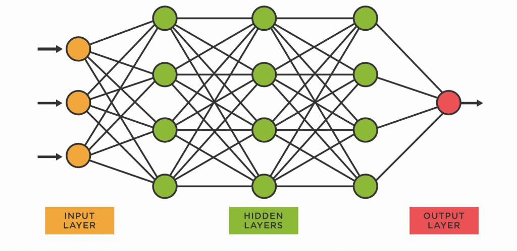
Neural networks are powerful because of the universal approximation theorem: a single hidden layer with enough neurons can approximate any continuous function on a compact set to arbitrary accuracy. In practice, depth (many layers) is more parameter-efficient than width for learning hierarchical features.

This library provides a minimal, statically-sized neural network framework designed for embedded inference — no heap allocation, no dynamic shapes, full compile-time dimension checking. The forward and backward passes described below are implemented; the parameter update loop that turns them into on-device training is roadmap N8/N9/N16 (see Model).

4.1.2 Mathematical Theory

4.1.2.1 Forward Propagation

Given \(L\) layers, the network computes:

\[a_0 = x\] \[z_\ell = W_\ell \, a_{\ell-1} + b_\ell, \quad \ell = 1, \ldots, L\] \[a_\ell = f_\ell(z_\ell)\] \[\hat{y} = a_L\]

where \(W_\ell \in \mathbb{R}^{n_\ell \times n_{\ell-1}}\) are weights, \(b_\ell \in \mathbb{R}^{n_\ell}\) are biases, and \(f_\ell\) is the activation function for layer \(\ell\).

4.1.2.2 Loss Function

Training minimizes a scalar loss \(\mathcal{L}(\hat{y}, y)\) that measures how far the prediction \(\hat{y}\) is from the target \(y\). Common choices (see Loss Functions):

4.1.2.3 Backpropagation

Backpropagation computes \(\nabla_\theta \mathcal{L}\) via the chain rule, working from the output layer backward. With \(g_L = \nabla_{a_L} \mathcal{L}\) and \(J_{f_\ell}\) the Jacobian of the activation:

\[\delta_\ell = J_{f_\ell}(z_\ell)^T g_\ell, \qquad g_{\ell-1} = W_\ell^T \delta_\ell\]

For element-wise activations \(J_{f_\ell}\) is diagonal and \(\delta_\ell = g_\ell \odot f_\ell'(z_\ell)\); for Softmax it is the \(O(n_\ell)\) product \(\delta_\ell = a_\ell \odot (g_\ell - \langle g_\ell, a_\ell \rangle)\) (see Activation Functions). The gradients with respect to the parameters are:

\[\frac{\partial \mathcal{L}}{\partial W_\ell} = \delta_\ell \, a_{\ell-1}^T, \qquad \frac{\partial \mathcal{L}}{\partial b_\ell} = \delta_\ell\]

4.1.2.4 Parameter Update

An optimizer uses the gradients to update the parameter vector \(\theta\):

\[\theta_{t+1} = \theta_t - \eta \, \nabla_\theta \mathcal{L}\]

where \(\eta\) is the learning rate. More sophisticated optimizers (momentum, Adam) modify this basic rule. With a mini-batch of \(B\) samples, \(\nabla_\theta \mathcal{L}\) is the average of the per-sample gradients.

4.1.3 Complexity Analysis

where \(P = \sum_\ell (n_\ell \cdot n_{\ell-1} + n_\ell)\) is the total parameter count. Both passes cost about one multiply-accumulate per weight, so a network with \(P = 10{,}000\) parameters needs on the order of \(10^4\) MACs per sample and pass.

4.1.4 Step-by-Step Walkthrough

Network: 2 inputs → 2 hidden (ReLU) → 1 output (Sigmoid), trained with binary cross-entropy on one XOR sample.

Architecture:

graph LR
    x1((x₁)) --> h1((h₁))
    x1 --> h2((h₂))
    x2((x₂)) --> h1
    x2 --> h2
    h1 --> y((ŷ))
    h2 --> y

Initial parameters:

\[W_1 = \begin{bmatrix} 0.2 & 0.4 \\ -0.3 & 0.1 \end{bmatrix}, \quad b_1 = \begin{bmatrix} 0.1 \\ 0.2 \end{bmatrix}, \quad W_2 = \begin{bmatrix} 0.5 & -0.4 \end{bmatrix}, \quad b_2 = [0]\]

Forward pass with input \(x = [1, 0]^T\), target \(y = 1\):

Backward pass (Sigmoid followed by BCE simplifies to \(\delta_2 = \hat{y} - y\)):

Update with \(\eta = 0.1\): \(W_2 \leftarrow [0.5139, -0.4]\), \(b_2 \leftarrow 0.0463\), \(W_{1,11} \leftarrow 0.2231\), \(b_{1,1} \leftarrow 0.1231\) (all other parameters have zero gradient). Repeating the forward pass gives \(\hat{y} = \sigma(0.2242) = 0.5558\) and \(\mathcal{L} = 0.5873\) — the loss decreased. Training repeats this step over all four XOR samples.

4.1.5 Pitfalls & Edge Cases

• Vanishing gradients. Deep networks with Sigmoid or Tanh activations suffer exponential gradient decay. Prefer ReLU-family activations in hidden layers.
• Exploding gradients. Large weights amplify gradients exponentially. Use proper weight initialization (Glorot for Sigmoid/Tanh, He \(\mathcal{N}(0, 2/n_{\text{in}})\) for ReLU) and gradient clipping.
• Dead neurons. ReLU neurons that receive only negative inputs output zero forever. Leaky ReLU mitigates this.
• Symmetric initialization. Identical initial weights make every neuron in a layer learn the same function; initial weights must break symmetry.
• Learning rate sensitivity. Too high → divergence; too low → no progress. Start with \(\eta = 0.01\) and adjust.
• Overfitting. Small embedded datasets are easily memorized. Apply regularization (L2 weight decay) on \(\theta\).
• Single precision. All arithmetic is 32-bit float: accumulations over many terms lose precision, and saturated Sigmoid/Softmax outputs round to exactly 0 or 1. Keep inputs normalised and use the numerically stable loss forms.

4.1.6 Variants & Generalizations

4.1.7 Applications

• Function approximation — Learning arbitrary input-output mappings from data.
• Classification — Mapping inputs to discrete categories (fault detection, gesture recognition).
• Regression — Predicting continuous values (sensor calibration, system identification).
• Control — Neural network policies for model-free or model-predictive control on embedded targets.
• Signal processing — Learned filters replacing hand-designed FIR/IIR chains.

4.1.8 Connections to Other Algorithms

graph TD
    NN["Neural Network"]
    Layer["Dense Layer"]
    Act["Activation Functions"]
    Loss["Loss Functions"]
    Opt["Optimizer"]
    Reg["Regularization"]
    Model["Model"]
    LR["Linear Regression"]

    Layer --> NN
    Act --> NN
    Loss --> NN
    Opt --> NN
    Reg --> NN
    NN --> Model
    NN -.->|"single layer, identity activation, MSE loss"| LR

4.2 Model (Sequential Composition)

4.2.1 Overview & Motivation

A model composes a sequence of layers — today dense layers — into a single function \(f_\theta: \mathbb{R}^n \to \mathbb{R}^m\). It:

1. Chains layers so the output of each feeds into the next (forward pass).
2. Propagates the output gradient backward through the chain (backward pass), returning \(\partial \mathcal{L} / \partial x\); each layer computes its own parameter gradients on the way.
3. Exports and imports all layer parameters as one flat vector \(\theta \in \mathbb{R}^P\).
4. Verifies dimensional compatibility at compile time: the model input size, every layer-to-layer interface and the model output size must agree, and there must be at least one layer.
5. Offers a parameter-space training step: an optimizer minimises a user-supplied objective \(J(\theta)\) over the flat parameter vector and the minimiser is loaded into the layers.

The model is fully statically typed — layer dimensions, parameter counts, and memory footprints are all known at compile time, enabling zero-overhead abstraction on embedded targets.

4.2.2 Mathematical Theory

4.2.2.1 Composition

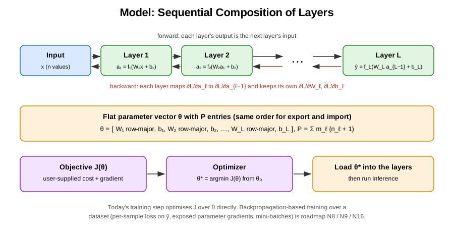
For \(L\) layers with transformations \(f_1, f_2, \ldots, f_L\):

\[\hat{y} = (f_L \circ f_{L-1} \circ \cdots \circ f_1)(x) = f_L(f_{L-1}(\ldots f_1(x) \ldots))\]

Each \(f_\ell\) is a dense layer: \(a_\ell = f_\ell(a_{\ell-1}) = \sigma_\ell(W_\ell a_{\ell-1} + b_\ell)\) with \(a_0 = x\), \(W_\ell \in \mathbb{R}^{m_\ell \times n_\ell}\) and \(n_{\ell+1} = m_\ell\).

4.2.2.2 Parameter Vector

All weights and biases are concatenated in layer order; each \(W_\ell\) is flattened row-major (row \(i\) = weights of output neuron \(i\)), followed by its bias:

\[\theta = [\, \operatorname{rows}(W_1),\ b_1,\ \operatorname{rows}(W_2),\ b_2,\ \ldots,\ \operatorname{rows}(W_L),\ b_L \,] \in \mathbb{R}^P, \qquad P = \sum_{\ell=1}^L m_\ell(n_\ell + 1)\]

Export and import use exactly this order, so exporting and re-importing is the identity.

4.2.2.3 Forward Pass (Chained Evaluation)

graph LR
    X["x ∈ ℝⁿ"] --> L1["Layer 1"] --> L2["Layer 2"] --> Ldots["⋯"] --> LL["Layer L"] --> Y["ŷ ∈ ℝᵐ"]

4.2.2.4 Backward Pass (Reverse Chain Rule)

Given \(g_L = \partial \mathcal{L} / \partial \hat{y}\), the layers are visited in reverse. Layer \(\ell\) receives \(g_\ell = \partial \mathcal{L} / \partial a_\ell\) and computes

\[\delta_\ell = J_{\sigma_\ell}(z_\ell)^T g_\ell, \qquad \nabla W_\ell = \delta_\ell\, a_{\ell-1}^T, \qquad \nabla b_\ell = \delta_\ell, \qquad g_{\ell-1} = W_\ell^T \delta_\ell\]

so each layer applies its own activation derivative before handing \(g_{\ell-1}\) to its predecessor. The model returns \(g_0 = \partial \mathcal{L} / \partial x\). The per-layer parameter gradients stay inside the layers; exporting them as a flat \(\nabla_\theta \mathcal{L}\) is roadmap N8.

4.2.2.5 Training Step (Parameter-Space Optimisation)

The training step takes an optimizer, an objective \(J: \mathbb{R}^P \to \mathbb{R}\) with its gradient \(\nabla J\), and a starting point \(\theta_0\):

\[\theta^* = \operatorname{Optimize}(J, \theta_0) \approx \arg\min_\theta J(\theta), \qquad \text{then load } \theta^* \text{ into the layers}\]

It does not iterate over a dataset and does not call the forward or backward pass: the objective must itself encode whatever it measures about \(\theta\) (for example a user-written empirical risk). If a per-sample loss is passed as \(J\), its argument is \(\theta\) and its target is a parameter vector — it regresses the parameters onto that target. End-to-end back-propagation training — per-sample loss on \(\hat{y}\) (N9), exported parameter gradients (N8) and a mini-batch gradient step (N16) — is on the roadmap.

graph LR
    J["Objective J(θ), ∇J(θ)"] --> OPT["Optimizer from θ₀"] --> TH["θ*"] --> SET["Load θ* into layers"]

4.2.3 Complexity Analysis

Forward and backward are linear in the total parameter count \(P\) (one multiply-accumulate per weight). The resident model is the sum of its layers — about \(2P\) values plus the activation caches for dense layers (see Dense Layer).

4.2.4 Step-by-Step Walkthrough

Model: 2 → 3 → 1. Layer 1 uses ReLU, layer 2 uses Sigmoid.

Compile-time verification chain:

Parameters (\(P = 3(2 + 1) + 1(3 + 1) = 13\)):

\[W_1 = \begin{bmatrix} -0.5 & 0.2 \\ 0.4 & 0.6 \\ 0.1 & 0.2 \end{bmatrix}, \quad b_1 = \begin{bmatrix} 0.1 \\ 0.1 \\ 0.1 \end{bmatrix}, \quad W_2 = \begin{bmatrix} 0.3 & 0.5 & 0.2 \end{bmatrix}, \quad b_2 = [0.03]\]

Forward pass with \(x = [1.0, 0.5]^T\):

Backward pass with loss gradient \(g_2 = \partial \mathcal{L} / \partial \hat{y} = [0.12]\):

Note where \(\text{ReLU}'(z_1)\) enters: inside layer 1’s own backward pass, not in layer 2’s.

4.2.5 Pitfalls & Edge Cases

• Dimension mismatch caught at compile time. If layer \(\ell\) outputs \(m\) values but layer \(\ell+1\) expects \(n \ne m\), compilation fails.
• Empty model. A model needs at least one layer; zero layers is rejected at compile time.
• Parameter ordering. Export and import must use the same concatenation order (layer order, row-major weights, then biases). A transposed flattening silently scrambles a model loaded from an external source.
• Training step is not back-propagation. It minimises \(J(\theta)\) exactly as supplied. It never sees training samples; if \(J\) is a per-sample loss, the “prediction” it compares against the target is the parameter vector itself. Use it only with an objective written over \(\theta\), until roadmap N8/N9/N16 add gradient export, a per-sample loss contract and a mini-batch step.
• Objective size. The objective’s dimension must equal the total parameter count \(P\); a mismatch is caught at compile time.
• Backward before forward. Each layer’s backward pass uses the caches of the last forward pass; the model backward pass must follow a forward pass on the same sample.
• Memory. Each dense layer keeps its parameters and a same-sized gradient buffer, so the resident model is about \(2P\) values plus activation caches; parameter export adds a transient \(P\)-sized vector. A model with \(P = 10{,}000\) float parameters needs roughly 80 KB resident, not 40 KB — allocate it statically rather than on a small task stack.

4.2.6 Variants & Generalizations

4.2.7 Applications

• Embedded inference — Parameters trained offline are imported once and only the forward pass runs at runtime.
• Gradient-based input sensitivity — The backward pass yields \(\partial \mathcal{L} / \partial x\) for saliency or for inverting a small model.
• Parameter-space fitting — Small problems where an objective over \(\theta\) can be written directly (e.g. matching a known parameter vector, or a hand-written empirical risk) can use the training step today.
• System identification and sensor fusion — Small models (2–3 layers) mapping sensor inputs to plant outputs or state estimates, trained offline today and on-device once roadmap N16 lands.

4.2.8 Connections to Other Algorithms

graph TD
    Model["Model"]
    Layer["Dense Layer"]
    Loss["Loss Functions"]
    Opt["Optimizer"]
    Reg["Regularization"]
    NN["Neural Network"]

    Layer --> Model
    Model --> Opt
    Loss --> Opt
    Reg --> Loss
    Model --> NN

5 References

• Abadi, M. et al., “TensorFlow: A system for large-scale machine learning”, OSDI, 2016.
• Bishop, C.M., Pattern Recognition and Machine Learning, Springer, 2006.
• Clevert, D.-A., Unterthiner, T., and Hochreiter, S., “Fast and accurate deep network learning by exponential linear units (ELUs)”, ICLR, 2016.
• Glorot, X. and Bengio, Y., “Understanding the difficulty of training deep feedforward neural networks”, AISTATS, 2010.
• Glorot, X., Bordes, A., and Bengio, Y., “Deep sparse rectifier neural networks”, AISTATS, 2011.
• Goodfellow, I., Bengio, Y., and Courville, A., Deep Learning, MIT Press, 2016.
• He, K., Zhang, X., Ren, S., and Sun, J., “Delving deep into rectifiers: Surpassing human-level performance on ImageNet classification”, ICCV, 2015.
• Lin, T.-Y. et al., “Focal loss for dense object detection”, ICCV, 2017.
• Nair, V. and Hinton, G.E., “Rectified linear units improve restricted Boltzmann machines”, ICML, 2010.
• Paszke, A. et al., “PyTorch: An imperative style, high-performance deep learning library”, NeurIPS, 2019.
• Rumelhart, D.E., Hinton, G.E., and Williams, R.J., “Learning representations by back-propagating errors”, Nature, 323, 1986.