Field-Oriented Control (FOC)
| Field | Value |
|---|---|
| Title | Field-Oriented Control (FOC) |
| Type | theory |
| Status | approved |
| Version | 1.0.0 |
| Component | foc |
| Date | 2025-01-01 |
Overview
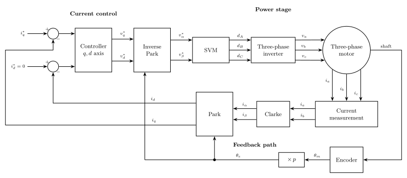
Field-Oriented Control (FOC) — also called vector control — is the standard high-performance control strategy for Permanent Magnet Synchronous Motors (PMSM) and Brushless DC motors (BLDC). Its central insight is that a three-phase AC motor can be controlled as simply as a DC motor if all quantities are expressed in a reference frame that rotates synchronously with the rotor flux.
In the rotating (dq) reference frame the three-phase stator currents reduce to two DC components: - \(i_d\) — the flux-producing (direct) component, nominally zero for maximum torque per ampere (MTPA). - \(i_q\) — the torque-producing (quadrature) component, directly proportional to electrical torque.
Current controllers in the rotating frame regulate these DC quantities without phase lag caused by the AC coupling. The inverse transforms and Space Vector Modulation (SVM) reconstruct the three-phase PWM duty cycles that drive the inverter.
Prerequisites
| Symbol | Meaning | Unit |
|---|---|---|
| \(R_s\) | Stator resistance per phase | Ω |
| \(L_s\) | Stator inductance per phase (assuming \(L_d = L_q\)) | H |
| \(\psi_f\) | Permanent magnet flux linkage | Wb |
| \(p\) | Number of pole pairs | — |
| \(\theta_e\) | Electrical rotor angle | rad |
| \(\theta_m\) | Mechanical rotor angle | rad |
| \(\omega_e\) | Electrical angular velocity (\(p \cdot \omega_m\)) | rad/s |
| \(V_{dc}\) | DC bus voltage | V |
| \(\tau_e\) | Electrical torque | N·m |
| \(1/\sqrt{3}\) | Reciprocal of \(\sqrt{3}\), ≈ 0.5774 | — |
The relationship between electrical and mechanical angles is:
\[ \theta_e = p \cdot \theta_m \]
Mathematical Foundation
1. PMSM Voltage Model (abc frame)
The PMSM stator voltage equations in the stationary abc reference frame are:
\[ v_a = R_s i_a + L_s \frac{di_a}{dt} + e_a \] \[ v_b = R_s i_b + L_s \frac{di_b}{dt} + e_b \] \[ v_c = R_s i_c + L_s \frac{di_c}{dt} + e_c \]
where \(e_a, e_b, e_c\) are the back-EMF voltages produced by the rotating permanent magnets:
\[ e_a = -\psi_f \omega_e \sin(\theta_e), \quad e_b = -\psi_f \omega_e \sin\!\left(\theta_e - \tfrac{2\pi}{3}\right), \quad e_c = -\psi_f \omega_e \sin\!\left(\theta_e + \tfrac{2\pi}{3}\right) \]
These equations are coupled through the mutual inductance and back-EMF, making direct control difficult. The Clarke and Park transforms decouple them into independently controllable quantities.
2. Clarke Transform — abc → αβ (Stationary Frame)
The Clarke transform projects the three-phase quantities onto a two-dimensional orthogonal stationary frame (\(\alpha\)–\(\beta\)). The amplitude-invariant form (factor \(\tfrac{2}{3}\)) preserves the physical voltage and current magnitudes:
\[ \begin{pmatrix} i_\alpha \\ i_\beta \end{pmatrix} = \frac{2}{3} \begin{pmatrix} 1 & -\tfrac{1}{2} & -\tfrac{1}{2} \\[4pt] 0 & \dfrac{\sqrt{3}}{2} & -\dfrac{\sqrt{3}}{2} \end{pmatrix} \begin{pmatrix} i_a \\ i_b \\ i_c \end{pmatrix} \]
For a balanced three-phase system (\(i_a + i_b + i_c = 0\)), the zero-sequence component vanishes and the transform simplifies. With only two current sensors measuring \(i_a\) and \(i_b\) (and \(i_c = -i_a - i_b\)):
\[ i_\alpha = i_a, \qquad i_\beta = \frac{i_a + 2\,i_b}{\sqrt{3}} \]
Verification: For a balanced current set \(i_a = I\cos\theta_e\), \(i_b = I\cos(\theta_e - \tfrac{2\pi}{3})\):
\[ i_\beta = \frac{I\cos\theta_e + 2I\!\left(-\tfrac{1}{2}\cos\theta_e + \tfrac{\sqrt{3}}{2}\sin\theta_e\right)}{\sqrt{3}} = \frac{I\sqrt{3}\sin\theta_e}{\sqrt{3}} = I\sin\theta_e \checkmark \]
The stator current space vector in the \(\alpha\)–\(\beta\) frame thus has magnitude \(I\) and rotates at \(\omega_e\): \(\mathbf{I}_s = i_\alpha + j\,i_\beta = I e^{j\theta_e}\).
Full three-sensor form (when all three currents are available):
\[ i_\alpha = \tfrac{2}{3}\!\left(i_a - \tfrac{1}{2}i_b - \tfrac{1}{2}i_c\right), \qquad i_\beta = \tfrac{1}{\sqrt{3}}\!\left(i_b - i_c\right) \]
3. Park Transform — αβ → dq (Rotating Frame)
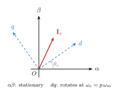
The Park transform rotates the \(\alpha\)–\(\beta\) space vector by \(-\theta_e\) into the rotor-fixed dq frame:
\[ \begin{pmatrix} i_d \\ i_q \end{pmatrix} = \begin{pmatrix} \cos\theta_e & \sin\theta_e \\ -\sin\theta_e & \cos\theta_e \end{pmatrix} \begin{pmatrix} i_\alpha \\ i_\beta \end{pmatrix} \]
\[ i_d = i_\alpha \cos\theta_e + i_\beta \sin\theta_e \] \[ i_q = -i_\alpha \sin\theta_e + i_\beta \cos\theta_e \]
For the balanced rotating current \(\mathbf{I}_s = I e^{j\theta_e}\):
\[ i_d + j\,i_q = I e^{j\theta_e} \cdot e^{-j\theta_e} = I \quad \Rightarrow \quad i_d = I,\ i_q = 0 \]
This confirms: when the current vector is aligned with the d-axis (rotor flux axis), \(i_q = 0\) (zero torque). When the current vector is 90° ahead of the rotor (MTPA), \(i_d = 0\) and \(i_q = I\) (maximum torque).
Inverse Park Transform (dq → αβ, for voltage reconstruction):
\[ \begin{pmatrix} v_\alpha \\ v_\beta \end{pmatrix} = \begin{pmatrix} \cos\theta_e & -\sin\theta_e \\ \sin\theta_e & \cos\theta_e \end{pmatrix} \begin{pmatrix} v_d \\ v_q \end{pmatrix} \]
\[ v_\alpha = v_d \cos\theta_e - v_q \sin\theta_e \] \[ v_\beta = v_d \sin\theta_e + v_q \cos\theta_e \]
4. PMSM Model in the dq Frame
After applying the Park transform, the PMSM voltage equations in the rotating dq frame become:
\[ v_d = R_s i_d + L_s \frac{di_d}{dt} - \omega_e L_s i_q \] \[ v_q = R_s i_q + L_s \frac{di_q}{dt} + \omega_e L_s i_d + \omega_e \psi_f \]
The cross-coupling terms \(\omega_e L_s i_q\) and \(\omega_e L_s i_d\) are decoupled by feed-forward compensation. The back-EMF term \(\omega_e \psi_f\) can also be added as a feed-forward. After decoupling, both d and q channels reduce to independent first-order RL systems:
\[ v_d' = R_s i_d + L_s \frac{di_d}{dt}, \qquad v_q' = R_s i_q + L_s \frac{di_q}{dt} \]
These are regulated by independent current controllers, one per dq axis.
5. Electrical Torque
The electromagnetic torque produced by the motor is:
\[ \boxed{\tau_e = \frac{3}{2}\, p\, \psi_f\, i_q} \]
Since \(\psi_f\) and \(p\) are motor constants, torque is directly proportional to \(i_q\). Setting the \(i_q\) reference from an outer speed or position loop gives a torque-current-mode inner loop — the fundamental advantage of FOC over scalar control.
The dq-axis current regulators are interchangeable at runtime. Gain
design and normalisation depend on the active algorithm — see the
current loop controller chapters in
documentation/theory/.
6. Space Vector Modulation (SVM)
SVM synthesises any reference voltage vector \(\mathbf{V}_{ref} = V_\alpha + j V_\beta\) as a time-average of the eight inverter states. The three-phase half-bridge inverter produces 8 switching states:
| Vector | Switches (A,B,C) | \(V_\alpha\) (normalised) | \(V_\beta\) (normalised) |
|---|---|---|---|
| \(V_0\) | (0,0,0) | 0 | 0 |
| \(V_1\) | (1,0,0) | \(\tfrac{2}{3}\) | 0 |
| \(V_2\) | (1,1,0) | \(\tfrac{1}{3}\) | \(\tfrac{1}{\sqrt{3}}\) |
| \(V_3\) | (0,1,0) | \(-\tfrac{1}{3}\) | \(\tfrac{1}{\sqrt{3}}\) |
| \(V_4\) | (0,1,1) | \(-\tfrac{2}{3}\) | 0 |
| \(V_5\) | (0,0,1) | \(-\tfrac{1}{3}\) | \(-\tfrac{1}{\sqrt{3}}\) |
| \(V_6\) | (1,0,1) | \(\tfrac{1}{3}\) | \(-\tfrac{1}{\sqrt{3}}\) |
| \(V_7\) | (1,1,1) | 0 | 0 |
The six active vectors (\(V_1\)–\(V_6\)) form a regular hexagon of circumradius \(\tfrac{2}{3}\) in these normalised units — that is the length of each vertex vector in the table above. The inscribed circle (maximum linear SVM range) is the hexagon’s apothem, \(\tfrac{2}{3}\cos 30^\circ = \tfrac{1}{\sqrt3} \approx 0.577\), corresponding to \(V_{dc}/\sqrt{3}\) in physical volts. The two agree: it is the circumradius that is \(\tfrac{2}{3}\), and reading that as the linear range overstates it by 15%.
See:
documentation/theory/images/svm_hexagon.svg (generated by
documentation/tools/generate_plots.gp)
Common-Mode Injection Method
This implementation uses the common-mode injection method (also called min-max injection), which avoids explicit sector detection. The three reference phase voltages are computed from \(V_\alpha, V_\beta\):
\[ v_A = V_\alpha \] \[ v_B = -\frac{V_\alpha}{2} + \frac{\sqrt{3}}{2}\,V_\beta \] \[ v_C = -\frac{V_\alpha}{2} - \frac{\sqrt{3}}{2}\,V_\beta \]
A common-mode offset is added to centre the signals within the PWM range:
\[ v_{common} = -\frac{\max(v_A, v_B, v_C) + \min(v_A, v_B, v_C)}{2} \]
Each phase duty cycle is then:
\[ d_k = \mathrm{clamp}\!\left(\frac{v_k + v_{common}}{\sqrt{3}} + 0.5,\ 0,\ 1\right), \quad k \in \{A, B, C\} \]
The factor \(1/\sqrt{3}\) in the duty cycle formula arises from the normalisation: at the hexagon boundary, the maximum phase voltage (after common-mode injection) is \(\sqrt{3}/2\) of the bus voltage, and the factor maps this to the [0, 1] duty cycle range centred at 0.5.
Advantages over sector-based SVM: - No angle or sector lookup required. - Identical results to classical SVM for three-phase symmetric loads. - Naturally handles over-modulation by saturation (clamping).
SVM Linear Modulation Region
The common-mode injection guarantees full hexagon utilisation. The maximum phase voltage in the linear region corresponds to modulation index \(m = 1.0\):
\[ |V_{ref}|_{max} = \frac{V_{dc}}{\sqrt{3}} \approx 0.577\, V_{dc} \]
Beyond this circle, one or more phases saturate (clamp) and the output enters over-modulation.
9. Trigonometric Lookup Table
The Park/inverse-Park transforms require \(\sin\theta_e\) and \(\cos\theta_e\) at the FOC control rate (20
kHz). To avoid calling sinf/cosf in the ISR:
- A 512-entry sine lookup table is stored in flash, 16-byte aligned for cache efficiency.
- The table covers one full electrical revolution:
LUT[k] = sin(2π·k/512). - Cosine is obtained by a 90° index offset:
cos(θ) = LUT[(k + 128) % 512]. - The electrical angle is mapped to a table index:
k = (uint16_t)(θ_norm * 512) & 0x1FF. - Angular range: angle is normalised to \([0, 1)\) representing \([0, 2\pi)\).
The fixed-step table introduces a bounded angle-quantisation error of at most \(\pi/512 \approx 0.35°\) when truncating to the nearest entry. The implementation interpolates linearly between adjacent entries, which bounds the amplitude error at \(\Delta^2/8 \approx 1.9 \times 10^{-5}\) instead. At 3000 rpm with \(p = 5\) the electrical angle advances \(\omega_e/20000 = 0.0785\ \text{rad} \approx 4.5°\) per step, roughly 6.4 table entries, so it is the interpolation rather than the table density that bounds the error.
Block Diagrams
Complete FOC Loop
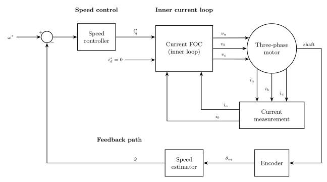
Speed Control Cascade
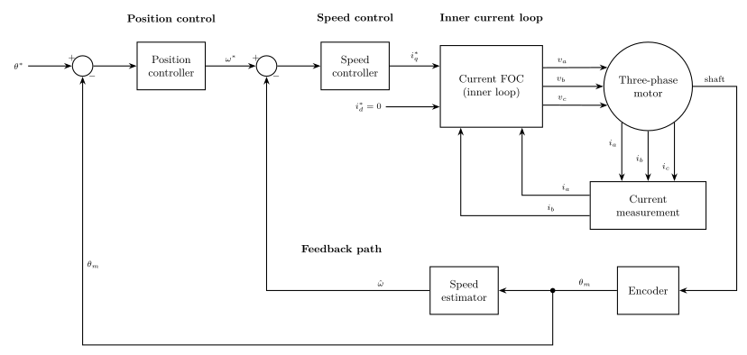
Position Control Cascade
Coordinate System Relationships
See also:
documentation/theory/images/foc_coordinates.svg and
documentation/theory/images/svm_hexagon.svg
Numerical Properties
| Property | Value / Condition |
|---|---|
| Control rate | 20 kHz (50 µs period) |
| Transform latency | < 20 CPU cycles (Clarke + Park combined) |
| LUT angle error | <= \(\pi/512 \approx 0.35°\) truncated; \(\approx 1.9\times10^{-5}\) interpolated |
| SVM duty resolution | \(2^{-16}\) of the period —
PhasePwmDutyCycles carries hal::DutyCycle (Q16
in a uint32_t) |
| Controller output | Applied \(v_{dq}\) limited to the unit circle \(\lVert v \rVert \le 1\); anti-windup on that limit |
| Torque linearity | \(\tau_e \propto i_q\) within MTPA region |
| Over-modulation | Clamp-based saturation; duty cycles bounded to [0, 1] |
| Gain normalisation | Physical V/A gains must be scaled by \(\sqrt{3}/V_{dc}\) to match per-unit SVM output |
| LUT memory | 512 × 4 bytes = 2048 bytes flash |
Sensitivity Analysis
| Parameter | Effect on Control Quality |
|---|---|
| \(R_s\) error | Current controller steady-state error (for non-integral controllers); compensated by integral term where present |
| \(L_s\) error | Controller bandwidth deviation; no steady-state error for integral-action controllers |
| \(\theta_e\) error | Cross-coupling between d and q axes; reduces torque at large error |
| \(V_{dc}\) variation | Affects gain normalisation; dynamic Vdc measurement recommended |
| ADC offset | Bias on \(i_d\), \(i_q\); must be calibrated at startup |
Worked Example
Motor parameters: \(R_s = 1.2\ \Omega\), \(L_s = 0.5\ \text{mH}\), \(p = 4\), \(\psi_f = 0.05\ \text{Wb}\), \(V_{dc} = 24\ \text{V}\).
Step 1 — Torque at \(i_q = 5\ \text{A}\):
\[\tau_e = \frac{3}{2} \times 4 \times 0.05 \times 5 = 1.5\ \text{N·m}\]
Step 2 — SVM for \(V_\alpha = 8\ \text{V}\), \(V_\beta = 5\ \text{V}\) (\(V_{dc} = 24\ \text{V}\)):
The modulator takes per-unit voltages, where \(1\ \text{pu} = V_{dc}/\sqrt{3} = 13.86\ \text{V}\). Since \(|V_{ref}| = \sqrt{64+25} \approx 9.43\ \text{V} < 13.86\ \text{V}\), the reference lies inside the linear region and no over-modulation clamping occurs.
\[v_\alpha^{pu} = 8/13.86 = 0.577,\quad v_\beta^{pu} = 5/13.86 = 0.361\] \[v_A = 0.577,\quad v_B = -0.289 + 0.866 \cdot 0.361 = 0.024,\quad v_C = -0.289 - 0.313 = -0.601\] \[v_{common} = -\frac{0.577 + (-0.601)}{2} = 0.012\] \[d_A = \mathrm{clamp}\!\left(\frac{0.589}{\sqrt{3}} + 0.5,\ 0,\ 1\right) = 0.840,\quad d_B = 0.521,\quad d_C = 0.160\]
Controller Slots
Each of the three control loops exposes a runtime-selectable controller slot. The active algorithm is configured via CLI or CAN without a firmware rebuild, and persists across power cycles via NVM.
- Current loop — regulates \(i_d\) and \(i_q\) at 20 kHz.
- Speed loop — regulates \(\omega\) at 1 kHz, produces \(i_q^*\) for the current loop.
- Position loop — regulates \(\theta\) at 1 kHz, produces \(\omega^*\) for the speed loop.
For design equations of each available algorithm, see the
per-algorithm theory chapters. An index of all algorithms with the
selection map and parameter sources is in
documentation/theory/advanced-controllers.md.
Plant models (current, speed, position) and discretisation are in
documentation/theory/foc-plant-models.md.
The runtime selection mechanism — heap-free variant storage,
type-aware dispatch, state gating, NVM persistence, and CLI/CAN
interface — is documented in
documentation/design/controller-selection.md.
Limitations & Assumptions
- Assumes: Surface-mounted PMSM with \(L_d = L_q\) (non-salient). For interior PMSM (\(L_d \neq L_q\)), MTPA condition changes and the torque equation gains an additional reluctance term.
- Assumes: Balanced three-phase supply (\(i_a + i_b + i_c = 0\)). If a phase is open, Clarke reduction from two sensors is invalid.
- Assumes: The electrical rotor angle \(\theta_e\) is accurately known (from encoder + alignment offset). Angle errors directly degrade torque production and can cause instability.
- Does not handle: Flux weakening above base speed (field weakening via non-zero \(i_d\)).
- Does not handle: Sensorless operation (this implementation uses an encoder for \(\theta_e\)).
References
- Krishnan, R. — Permanent Magnet Synchronous and Brushless DC Motor Drives, CRC Press, 2010.
- Holmes, D.G. & Lipo, T.A. — Pulse Width Modulation for Power Converters, IEEE Press / Wiley, 2003.
- Bose, B.K. — Modern Power Electronics and AC Drives, Prentice Hall, 2002.
- Texas Instruments Application Report SPRAA76A — Adjusted Space Vector Pulse Width Modulation for Voltage Source Inverters, 2005.