Electrical Parameters Identification — Resistance and Inductance
| Field | Value |
|---|---|
| Title | Electrical Parameters Identification — R and L |
| Type | theory |
| Status | approved |
| Version | 2.1.0 |
| Component | service-electrical-ident |
| Date | 2026-09-21 |
Overview
FOC performance depends directly on accurate stator resistance \(R_s\) and inductance \(L_s\). These parameters are used to: 1. Design the PI current controller gains (\(K_p = L_s \omega_{bw}\), \(K_i = R_s \omega_{bw}\)). 2. Implement feed-forward decoupling of the dq cross-coupling terms. 3. Estimate motor temperature from measured \(R_s\) (since \(R_s \propto T\)).
Two complementary offline identification methods are used, one for each parameter:
- Resistance — DC voltage step: steady-state V/I gives \(R_s\) directly. Accurate for any motor.
- Inductance — HF sinusoidal injection: synchronous demodulation of the current response at the injection frequency extracts Im(Z) and thus \(L_s\). Suitable for low-resistance motors where the time-constant method fails.
The reason two separate methods are needed is a fundamental signal-conditioning problem. At the 700 Hz injection frequency the ratio \(\omega L_s / R_s\) is 7 for the Anaheim BLY172S-24V-4000 (\(R_s = 0.405\,\Omega\), \(L_s = 0.64\,\text{mH}\)) and 2.4 for the Teknic M-2310P-LN-04K (\(R_s = 0.36\,\Omega\), \(L_s = 0.20\,\text{mH}\)), so resistance is 14 % and 38 % of the impedance.
For lower-resistance windings that share falls below 5 %, and any small phase error drowns the R signal entirely. The time-constant method (section 4 of version 1.0) likewise fails because \(\tau = L_s/R_s\) is 1.6 ms for the Anaheim and 0.56 ms for the Teknic, 16 and 5.6 samples at 10 kHz — too few for threshold-based detection through a filter of comparable length.
Each parameter is therefore extracted using the technique that makes it the dominant signal.
Prerequisites
| Symbol | Meaning | Unit |
|---|---|---|
| \(R_s\) | Stator resistance per phase | Ω |
| \(L_s\) | Stator inductance (\(L_d\), assuming surface PMSM) | H |
| \(V_{step}\) | DC step terminal voltage | V |
| \(I_{ss}\) | Steady-state current after DC step | A |
| \(f_{inj}\) | Sinusoidal injection frequency | Hz |
| \(\omega\) | Angular injection frequency = \(2\pi f_{inj}\) | rad/s |
| \(V_{inj}\) | Terminal sinusoidal injection amplitude | V |
| \(f_s\) | Sampling frequency (10 kHz) | Hz |
| \(T_s\) | Sampling period = \(1/f_s\) | s |
| \(N\) | Goertzel block length = \(N_{periods} \times N_{spp}\) | samples |
| \(N_{spp}\) | Samples per injection period = \(\text{round}(f_s / f_{inj})\) | samples |
| \(k\) | Goertzel bin index = \(N_{periods}\) | — |
| \(d\) | ADC pipeline delay | samples |
| \(a_d, b_d\) | ZOH coefficients: \(a_d = e^{-R_s T_s/L_s}\), \(b_d=(1-a_d)/R_s\) | — |
Mathematical Foundation
1. Terminal Excitation and Winding Factor
Both procedures apply voltage across one terminal versus the other two shorted together. For a wye machine, terminal A sees \(R_s\) in series with the other two in parallel; for delta it sees two windings in parallel:
\[ R_{terminal} = \begin{cases} \tfrac{3}{2} R_s & \text{wye} \\[2pt] \tfrac{1}{2} R_s & \text{delta} \end{cases}, \qquad L_{terminal} = \begin{cases} \tfrac{3}{2} L_s & \text{wye} \\[2pt] \tfrac{1}{2} L_s & \text{delta} \end{cases} \]
The same topology factor applies to both parameters. The applied voltage is the differential duty \((D_{test} - D_{neutral}) \cdot V_{dc}\) for the DC step, and for the sinusoidal injection the Clarke inverse of \(\{v, 0\}\) maps to three-phase duties \(\{v, -v/2, -v/2\}\) (phases relative to midpoint), which produces a terminal A-to-BC amplitude of \(v \cdot 0.75 \cdot V_{dc}\).
2. Resistance — DC Voltage Step
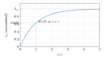
A known DC voltage \(V_{step}\) is held on the winding until the current reaches steady state (\(\gg 5\tau\)). At steady state all \(L\,\text{d}i/\text{d}t\) terms vanish:
\[ \boxed{R_s = \frac{V_{step}}{I_{ss}} \cdot \frac{1}{F_{terminal}}} \]
where \(F_{terminal}\) is the winding topology factor above and \(I_{ss}\) is the mean of the last 10 % of the sample buffer.
Why this fails for L: the DC step reveals only the time constant \(\tau = L_s/R_s\). For the Anaheim BLY172S (\(L_s = 0.64\,\text{mH}\), \(R_s = 0.405\,\Omega\)) \(\tau = 1.58\,\text{ms}\), which spans only 16 samples at 10 kHz, and for the Teknic M-2310P (\(0.20\,\text{mH}\), \(0.36\,\Omega\)) 5.6 samples. A 5-sample moving average and a single-sample crossing threshold cannot resolve such a narrow transient accurately. Inductance is therefore obtained by a separate frequency-domain method.
DC Step Response
3. Inductance — HF Sinusoidal Injection
3.1 Why Goertzel?
The inductance estimator must extract the amplitude and phase of the current response at exactly one known frequency. Several approaches were considered:
| Approach | Why rejected |
|---|---|
| Full FFT | Computes all bins; requires an N-sample RAM buffer (280–2000 samples = 1–8 kB); no embedded heap |
| Manual I/Q accumulation (\(\Sigma i \cdot \sin\), \(\Sigma i \cdot \cos\)) | Equivalent mathematically, but requires running \(\sin\) / \(\cos\) generation at every ISR sample (two trig calls per sample in the hot path) |
| Cross-correlation with stored reference | Requires storing the reference sinusoid — another N-sample buffer |
| Lock-in amplifier (hardware) | Purely analog; not applicable in software |
The Goertzel algorithm is a two-pole recursive filter:
s[n] = x[n] + 2·cos(ω₀)·s[n−1] − s[n−2]It accumulates the single-bin DFT coefficient \(X[k] = \sum_{n=0}^{N-1} x[n]\,e^{-j2\pi
kn/N}\) using only three state variables (\(s_1\), \(s_2\), sample count). It is streaming (one
sample at a time), needs no stored reference, and delivers an exact
complex result when Ready(). For N = 280 samples at 700 Hz,
it uses 12 bytes of working state versus 1.1 kB for an I/Q reference
buffer.
Exact bin alignment: the block size is chosen as \(N = N_{periods} \times N_{spp}\) and the Goertzel bin as \(k = N_{periods}\), so exactly \(N_{periods}\) complete injection cycles fit in the window. Any mismatch between injection frequency and analysis bin causes spectral leakage that biases \(\text{Im}(Z)\). The implementation snaps the injection to \(f_{inj}^{exact} = f_s / N_{spp}\) (nearest integer-sample-per-period frequency) to eliminate leakage entirely.
3.2 Injection and Demodulation
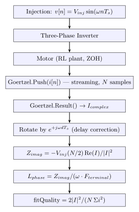
The sinusoidal voltage \(v[n] = V_{inj} \sin(\omega n T_s)\) is injected on the alpha axis only (beta = 0), keeping net electromagnetic torque at zero so the rotor remains stationary.
Over the measurement window, the Goertzel accumulates the current response and returns
\[ I_{Goertzel} = \sum_{n=0}^{N-1} i[n]\,e^{-j\omega n T_s} \]
For a sinusoidal current \(i[n] = I_0 \sin(\omega n T_s + \phi)\), this gives \(I_{Goertzel} = -j(N/2)\,I_0\,e^{-j\phi}\).
The voltage phasor at the same bin is \(V_{Goertzel} = -j(N/2)\,V_{inj}\) (for a sine input). The terminal impedance is then:
\[ Z_{terminal} = \frac{V_{Goertzel}}{I_{Goertzel}} \]
For an RL circuit, \(\text{Im}(Z) = \omega L_{terminal}\), so:
\[ \boxed{L_s = \frac{\text{Im}(Z_{terminal})}{\omega \cdot F_{terminal}}} \]
In practice, the full complex division reduces to:
\[ Z_{imag} = -\frac{V_{inj} \cdot N/2 \cdot \text{Re}(I_{corrected})}{|I_{corrected}|^2} \]
where \(I_{corrected}\) is the delay-compensated Goertzel result (see section 3.3).
3.3 ZOH Discretisation Bias
The sampler is a zero-order-hold (ZOH), not a true continuous-time integrator. At 10 kHz sampling, the ZOH introduces a systematic bias in \(\text{Im}(Z)\):
\[ Z_{ZOH} = \frac{1 - a_d\,e^{-j\omega T_s}}{b_d} \quad \Longrightarrow \quad \text{Im}(Z_{ZOH}) = \frac{a_d \sin(\omega T_s)}{b_d} \]
The fractional error in \(L_s\) relative to the continuous-time value scales approximately as \(R_s T_s / L_s\):
| Motor | \(R_s T_s / L_s\) | ZOH bias in \(L_s\) (estimate) | Measured in SIL |
|---|---|---|---|
| Anaheim BLY172S-24V-4000 (terminal) | 0.063 | ≈ 3 % | −6 % |
| Generic (R=0.5 Ω, L=0.5 mH terminal) | 0.10 | ≈ 5 % | |
| Teknic M-2310P-LN-04K (terminal) | 0.18 | ≈ 9 % | −15.5 % |
The terminal factor cancels in the ratio, so it is the per-phase \(R_s / L_s\) that sets the bias. The measured column is the software-in-the-loop identification against the exact plant, whose whole-percent duty quantises the 15 % injection and adds to the ZOH term; the estimate reads low in both cases. For the Anaheim motor the error is within calibration tolerance; for the Teknic it is not negligible. A correction using the already-measured \(R_s\) and \(b_d\) can be applied post-hoc; it is not implemented today.
3.4 ADC Delay Correction
The ADC delivers current sample \(i[k]\) that was measured from the voltage applied at step \(k-d\) (typically \(d = 1\) sample due to ISR pipeline latency). This introduces a phase lag of \(\omega \cdot d \cdot T_s\) on the Goertzel result. Correcting it requires a single complex rotation applied after the Goertzel completes — no per-sample cost:
\[ I_{corrected} = I_{Goertzel} \cdot e^{+j\omega d T_s} \]
Applying the correction with the wrong sign doubles the delay error instead of cancelling it.
3.5 Coherence (fitQuality)
The ratio of signal power at \(f_{inj}\) to total current power is a dimensionless quality metric:
\[ \text{fitQuality} = \frac{2\,|I_{Goertzel}|^2}{N \cdot \sum_{n} i[n]^2} \quad \in [0, 1] \]
This equals 1.0 for a pure sinusoid at \(f_{inj}\) and drops toward zero when the current contains large non-injection-frequency content (noise, harmonics, rotor motion). Calibration is rejected when fitQuality falls below 0.5.
3.6 Hardware Note — Dead-Time Voltage Error
Inverter dead-time introduces a voltage error at the switching frequency that corrupts the injection signal. At 500 ns dead-time and 20 kHz PWM the error voltage is approximately \(2 \cdot t_{dt} \cdot f_{sw} \cdot V_{dc} \approx 0.48\,\text{V}\) at \(V_{dc} = 24\,\text{V}\). At 10 % injection (\(V_{inj} = 2.4\,\text{V}\)) this represents 20 % distortion; at 15 % (\(V_{inj} = 3.6\,\text{V}\)) it falls to 13 %. The minimum recommended injection voltage is 15 % of bus to keep dead-time distortion below 15 % of the injected signal. The software model does not reproduce dead-time; simulation results will be optimistic relative to hardware.
Signal Flow
4. Pole Pair Estimation
The number of electrical cycles per mechanical revolution equals the number of pole pairs \(p\). During the pole-pair electrical-angle sweep, the motor is driven through exactly \(N_{rev}\) electrical revolutions over \(12 \cdot N_{rev}\) steps. The total mechanical angle \(\Delta\theta_{mech}\) is accumulated from the encoder. The pole pairs are:
\[ p = \text{round}\!\left(\frac{2\pi N_{rev}}{\Delta\theta_{mech,total}}\right) \]
If the total mechanical rotation is below \(\pi/2\) (rotor not following the field), the result is absent.
Numerical Properties
| Property | DC Step (R) | HF Sinusoidal (L) |
|---|---|---|
| Sampling rate | 10 kHz | 10 kHz |
| Excitation | Differential DC step (testVoltage) | Alpha-axis sine at \(f_{inj}\) (default 700 Hz) |
| Working memory | 5-sample deque + 123-sample buffer | 3 floats (Goertzel state) + sumSquared + sampleCount |
| Settling required | \(\geq 5\tau\) before R is valid | warmupPeriods full cycles (rotor transient decay) |
| Result quality gate | \(I_{ss} > 0\) | fitQuality \(\geq 0.5\) |
| Min injection voltage | — | \(\geq 15\%\) bus (dead-time floor on hardware) |
| ZOH bias in L | — | \(\approx R_s T_s / L_s\) fractional underestimate |
Limitations
- Assumes rotor stationary. Any rotor motion during either procedure overlays back-EMF on the measurements.
- Assumes magnetic linearity. Injection current must stay below the saturation onset of the winding.
- Assumes \(L_d \approx L_q\). For interior PMSM a separate \(L_q\) measurement is required.
- ZOH bias grows with \(R_s T_s / L_s\): about 3 % for the Anaheim BLY172S and 9 % for the Teknic M-2310P at 10 kHz.
- Dead-time on real hardware distorts the sinusoidal injection; models and simulation are optimistic.
- Temperature: \(R_s\) measurement is valid at the moment of identification only.
References
- Rauf, A. et al. — “Online Identification of PMSM Parameters Based on Extended Kalman Filter”, IEEE Transactions on Industrial Electronics, 2019.
- Underwood, S.J. & Husain, I. — “Online Parameter Estimation and Adaptive Control of PMSM”, IEEE Transactions on Industrial Electronics, 2010.
- Texas Instruments Application Report SPRABV5 — Motor Control in Embedded Applications, 2018.