Mechanical Parameters Identification — Friction and Inertia
| Field | Value |
|---|---|
| Title | Mechanical Parameters Identification — Friction and Inertia |
| Type | theory |
| Status | approved |
| Version | 1.0.0 |
| Component | service-mechanical-ident |
| Date | 2025-01-01 |
Overview
Accurate knowledge of the mechanical plant parameters — rotor moment of inertia \(J\), viscous friction coefficient \(B\), and Coulomb (static) friction torque \(\tau_0\) — is required to design an optimal speed or position loop, to implement feed-forward compensation, and to estimate system health over time.
This identification procedure uses Recursive Least Squares (RLS) to fit the parameters of Newton’s rotational equation of motion to real-time measurements of torque (estimated from \(i_q\)) and speed/ acceleration (derived from the encoder). RLS operates online in every control cycle, converging to the true parameters as the motor is excited with varying speed profiles.
Prerequisites
| Symbol | Meaning | Unit |
|---|---|---|
| \(J\) | Rotor moment of inertia | kg·m² |
| \(B\) | Viscous friction coefficient | N·m·s/rad |
| \(\tau_0\) | Coulomb friction (static offset) | N·m |
| \(\tau_e\) | Electrical (motor) torque = \(\frac{3}{2}p\psi_f i_q\) | N·m |
| \(\tau_{load}\) | External load torque (treated as disturbance) | N·m |
| \(\omega\) | Rotor mechanical angular velocity | rad/s |
| \(\alpha\) | Rotor angular acceleration = \(\dot\omega\) | rad/s² |
| \(\mathbf{\theta}\) | Parameter vector \([J,\ B,\ \tau_0]^T\) | mixed |
| \(\mathbf{\phi}\) | Regressor vector \([\alpha,\ \omega,\ 1]^T\) | mixed |
| \(\lambda\) | RLS forgetting factor | — |
| \(\mathbf{P}\) | Error covariance matrix (3×3) | — |
| \(\mathbf{K}\) | Kalman gain vector (3×1) | — |
Mathematical Foundation
1. Mechanical Equation of Motion
The PMSM rotor dynamics are described by Newton’s second law for rotation. Assuming viscous friction and a constant Coulomb friction offset:
\[ \tau_e = J\dot\omega + B\omega + \tau_0 + \tau_{load} \]
Ignoring unmeasured load torque (treated as noise by the estimator), this becomes a linear regression:
\[ \tau_e = \mathbf{\phi}^T \mathbf{\theta} \]
where:
\[ \mathbf{\phi} = \begin{pmatrix}\dot\omega \\ \omega \\ 1\end{pmatrix}, \qquad \mathbf{\theta} = \begin{pmatrix}J \\ B \\ \tau_0\end{pmatrix} \]
The regression form makes the parameter vector \(\mathbf{\theta}\) directly estimable from measured input-output data \((\mathbf{\phi}, \tau_e)\) using least squares.
2. Batch Least Squares (Background)
If \(N\) measurements are collected: \[ \mathbf{y} = \mathbf{\Phi}\,\mathbf{\theta} + \mathbf{e} \]
where \(\mathbf{y} \in \mathbb{R}^N\) is the torque sequence, \(\mathbf{\Phi} \in \mathbb{R}^{N \times 3}\) is the regressor matrix, and \(\mathbf{e}\) is noise. The ordinary least-squares solution is:
\[ \hat{\mathbf{\theta}} = (\mathbf{\Phi}^T\mathbf{\Phi})^{-1}\mathbf{\Phi}^T\mathbf{y} \]
This requires storing all \(N\) measurements and inverting a 3×3 matrix. RLS computes the same result recursively, processing one sample at a time with \(O(n^2)\) cost where \(n=3\) is the number of parameters.
3. Recursive Least Squares — Derivation
Define the weighted least-squares cost with exponential forgetting factor \(\lambda \in (0, 1]\):
\[ J_N = \sum_{k=1}^{N} \lambda^{N-k}\!\left(\tau_e[k] - \mathbf{\phi}[k]^T\hat{\mathbf{\theta}}\right)^2 \]
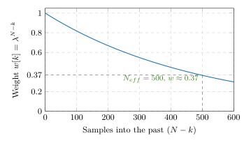
The exponential weight \(\lambda^{N-k}\) discounts older measurements, giving the estimator a finite effective memory window of \(\approx 1/(1-\lambda)\) samples.
Applying the matrix inversion lemma (Woodbury identity) to the recursive update of \(\mathbf{P}_N = (\sum_{k=1}^N \lambda^{N-k}\mathbf{\phi}[k]\mathbf{\phi}[k]^T)^{-1}\) yields:
\[ \boxed{ \mathbf{K}[n] = \frac{\mathbf{P}[n-1]\,\mathbf{\phi}[n]}{\lambda + \mathbf{\phi}[n]^T\mathbf{P}[n-1]\,\mathbf{\phi}[n]} } \]
\[ \boxed{ \hat{\mathbf{\theta}}[n] = \hat{\mathbf{\theta}}[n-1] + \mathbf{K}[n]\!\left(\tau_e[n] - \mathbf{\phi}[n]^T\hat{\mathbf{\theta}}[n-1]\right) } \]
\[ \boxed{ \mathbf{P}[n] = \frac{1}{\lambda}\!\left(\mathbf{I} - \mathbf{K}[n]\,\mathbf{\phi}[n]^T\right)\mathbf{P}[n-1] } \]
The scalar \(e[n] = \tau_e[n] - \mathbf{\phi}[n]^T\hat{\mathbf{\theta}}[n-1]\) is called the innovation (prediction error). The gain \(\mathbf{K}\) weights how much to move the estimate in response to the innovation.
Forgetting Factor
For \(\lambda = 1\) (no forgetting) the RLS is equivalent to batch LS over the entire history. For \(\lambda < 1\) older data is exponentially discounted. The effective memory window is:
\[ N_{eff} = \frac{1}{1 - \lambda} \]
With \(\lambda = 0.9995\) — the
value
RealTimeFrictionAndInertiaEstimator::defaultForgettingFactor
carries — \(N_{eff} = 2000\) samples,
two seconds at the 1 kHz outer-loop rate. The memory has to span more
than one level of the excitation: within a single plateau the intercept
and the speed column are collinear, so a memory shorter than a plateau
(the 200 ms that \(\lambda = 0.995\)
gave against a 250 ms dwell) can never separate \(B\) from \(\tau_0\), and the online friction estimate
wandered around zero.
A forgetting factor also inflates the covariance in any direction the
regressor does not excite, by \(\lambda^{-1}\) per update. A plateau still
informs \(B\) and \(\tau_0\) but not \(J\), so the online estimator takes plateau
samples only while the covariance trace stays under a ceiling, and
accelerating samples always; see
documentation/design/service-mechanical-ident.md §
Persistence of Excitation.
4. Torque and Kinematics Estimation
Torque: The motor torque is estimated from the q-axis current:
\[ \tau_e = \frac{3}{2}\,p\,\psi_f\,i_q = K_T\, i_q \]
The torque constant \(K_T = \frac{3}{2}p\psi_f\) must be known from the electrical identification stage or from the motor datasheet.
Speed: Measured directly from the encoder as:
\[ \omega[n] = \frac{\theta_m[n] - \theta_m[n-1]}{T_s} \]
Acceleration: Estimated by finite difference of speed:
\[ \dot\omega[n] = \frac{\omega[n] - \omega[n-1]}{T_s} \]
The double finite difference amplifies measurement noise. A low-pass filter (e.g. moving average) on \(\omega\) before differentiation reduces this effect at the cost of bandwidth.
4.1 The online form: window averages, not samples
At the 20 kHz control rate a single sample of \(i_q\) and a second difference of the encoder describe the same instant closely enough. At the 1 kHz outer-loop rate they do not. The speed difference \(\omega[n] - \omega[n-1]\) of two window-mean speeds is a triangular average of the acceleration centred one outer sample earlier than the instantaneous current \(i_q[n]\) it used to be regressed against. With the speed loop’s transients decaying at \(\sigma \approx 400\) rad/s that misalignment scales the identified inertia by about \(e^{-\sigma T} \approx 0.67\) — the 26–33 % low reading the SIL first measured.
The online estimator therefore regresses quantities the control interrupt integrates over each outer period \(T\). With \(\bar\omega_k = (\theta_k - \theta_{k-1})/T\) the window-mean speed and \(\bar i_{q,k}\) the window-mean current (trapezoidal over the interrupt’s samples), the momentum balance integrated across two windows gives, to second order,
\[ \boxed{K_T\,\frac{\bar i_{q,k} + \bar i_{q,k-1}}{2} = J\,\frac{\bar\omega_k - \bar\omega_{k-1}}{T} + B\,\frac{\bar\omega_k + \bar\omega_{k-1}}{2} + \tau_0} \]
Both sides now describe the same span, and the switching ripple is averaged out rather than sampled. Two details keep the window honest. The angle is latched by the interrupt at the window boundary: the outer loop can start a tick late, and differencing the angle it finds then measured 19- or 21-tick spans as if they were 20, an acceleration noise of some 2000 rad/s² that biased \(J\) toward zero exactly as the misalignment did. And the regression runs in milli-newton-metres against micro-unit \(J\) and \(B\), so its three columns are of order one on these rotors.
5. Convergence Criteria
The offline identification has converged to reliable estimates when:
Innovation is small: \(|e[n]| = |\tau_e[n] - \mathbf{\phi}[n]^T\hat{\mathbf{\theta}}[n]| < \epsilon_e\)
This indicates the model fits the data well (low residual error).
Gain trace is small: \(\mathrm{tr}(\mathbf{K}[n]) < \epsilon_K\)
This indicates the covariance has collapsed (the estimator is no longer updating significantly), i.e. the estimate has stabilised.
The two thresholds in use: \(\epsilon_e = 10^{-4}\) and \(\epsilon_K = 10^{-2}\).
The gain trace criterion is a proxy for \(\mathrm{tr}(\mathbf{P}[n])\) shrinking, which proves that \(\hat{\mathbf{\theta}}[n]\) has converged to a minimum-variance estimate given the data.
Both procedures also require the observations to have included enough accelerating samples and to span more than one speed (a quarter of the fastest seen), which is what identifies \(J\) and separates \(B\) from \(\tau_0\) respectively.
The online estimator does not use the instantaneous innovation: 0.1 mN·m sits under the torque ripple any real drive has, so it was met by chance. It publishes once it has taken a thousand observations and its exponentially averaged residual power is under 1 % of the averaged output power — the fit explains the torque it sees.
6. Observability Requirement
RLS identifies \(J\), \(B\), and \(\tau_0\) simultaneously only if the regressor matrix \(\mathbf{\Phi}\) is persistently exciting of order 3 — i.e. the columns \([\dot\omega, \omega, 1]\) are linearly independent over the observation window. In practice this requires:
- \(\dot\omega \neq 0\): the motor must accelerate and decelerate (constant-speed operation cannot identify \(J\)).
- \(\omega\) must vary over a sufficient range to separate \(B\omega\) from \(\tau_0\).
- Both positive and negative torques should appear if possible (else \(\tau_0\) is poorly identified).
A typical identification profile: triangular speed reference — ramp up, hold briefly, ramp down — repeated \(\ge 2\) times.
Block Diagrams
RLS Signal Flow

Effective Memory Window (Forgetting Factor)
Numerical Properties
| Property | Value / Condition |
|---|---|
| Parameter vector size | 3: \([J,\ B,\ \tau_0]^T\) |
| Covariance matrix | \(3\times 3\) symmetric positive definite |
| Forgetting factor (online) | \(\lambda = 0.9995\) |
| Effective window (online) | \(N_{eff} = 1/(1-\lambda) = 2000\) outer-loop samples |
| Convergence check \(\epsilon_e\) | \(10^{-4}\) (innovation threshold) |
| Convergence check \(\epsilon_K\) | \(10^{-2}\) (gain trace threshold) |
| RLS per-step cost | \(O(n^2) = O(9)\) — 9 multiply-add ops for \(n=3\) |
| Numerical stability | \(\mathbf{P}\) can become indefinite; use regularisation if \(\lambda < 1\) for long runs |
| Initialisation | \(\mathbf{P}_0 = \alpha_0 \mathbf{I}\), \(\hat{\mathbf{\theta}}_0 = \mathbf{0}\) |
Sensitivity Analysis
| Source of Error | Effect |
|---|---|
| \(K_T\) error | All parameters scaled proportionally (\(\tau_e\) is biased) |
| Encoder quantisation | Noise on \(\alpha\); use long averaging window |
| Constant-speed operation | \(J\) unidentifiable (\(\dot\omega = 0\) makes regressor rank-deficient) |
| Very short identification time | \(\mathbf{P}\) not collapsed; noisy estimates |
| \(\lambda\) too large | Slow convergence to parameter changes |
| \(\lambda\) too small | Noisy, unstable estimates at steady state |
Worked Example
Motor: \(J = 2 \times 10^{-4}\ \text{kg·m}^2\), \(B = 5 \times 10^{-4}\ \text{N·m·s/rad}\), \(\tau_0 = 0.01\ \text{N·m}\), \(K_T = 0.3\ \text{N·m/A}\), \(f_s = 1\ \text{kHz}\).
Regressor at one sample with \(\dot\omega = 50\ \text{rad/s}^2\), \(\omega = 100\ \text{rad/s}\), \(i_q = 2\ \text{A}\):
\[ \mathbf{\phi} = \begin{pmatrix}50\\ 100\\ 1\end{pmatrix}, \quad \tau_e = K_T\, i_q = 0.3 \times 2 = 0.6\ \text{N·m} \]
True output:
\[ \mathbf{\phi}^T\mathbf{\theta}_{true} = 50 \times 2\times10^{-4} + 100 \times 5\times10^{-4} + 0.01 = 0.01 + 0.05 + 0.01 = 0.07\ \text{N·m} \]
The difference 0.6 − 0.07 = 0.53 N·m is the load torque \(\tau_{load}\), which becomes the innovation residual from the estimator perspective — it will be treated as noise and averaged out over \(N_{eff}\) samples.
Limitations & Assumptions
- Assumes: \(\tau_{load}\) is zero mean over the effective window (i.e. no sustained external load that would be attributed to \(\tau_0\) or \(J\)).
- Assumes: Motor torque constant \(K_T\) is known a priori (from electrical identification).
- Assumes: The mechanical system is linear in \(J\), \(B\), \(\tau_0\) — nonlinear effects (e.g. position-dependent cogging, Stribeck friction) are not modelled.
- Does not handle: Rapidly varying \(J\) (e.g. moving load). The \(N_{eff} = 200\) sample window means changes faster than 200 ms update time are tracked with lag.
- Does not handle: Identification in the presence of external vibration or impact loads.
References
- Ljung, L. — System Identification: Theory for the User, 2nd ed., Prentice Hall, 1999.
- Åström, K.J. & Wittenmark, B. — Adaptive Control, 2nd ed., Addison-Wesley, 1995.
- Kim, J.-H. et al. — “Online Parameter Identification of PMSM Using Recursive Least-Squares Algorithm”, IEEE International Electric Machines and Drives Conference, 2007.